Space and Time Complexity

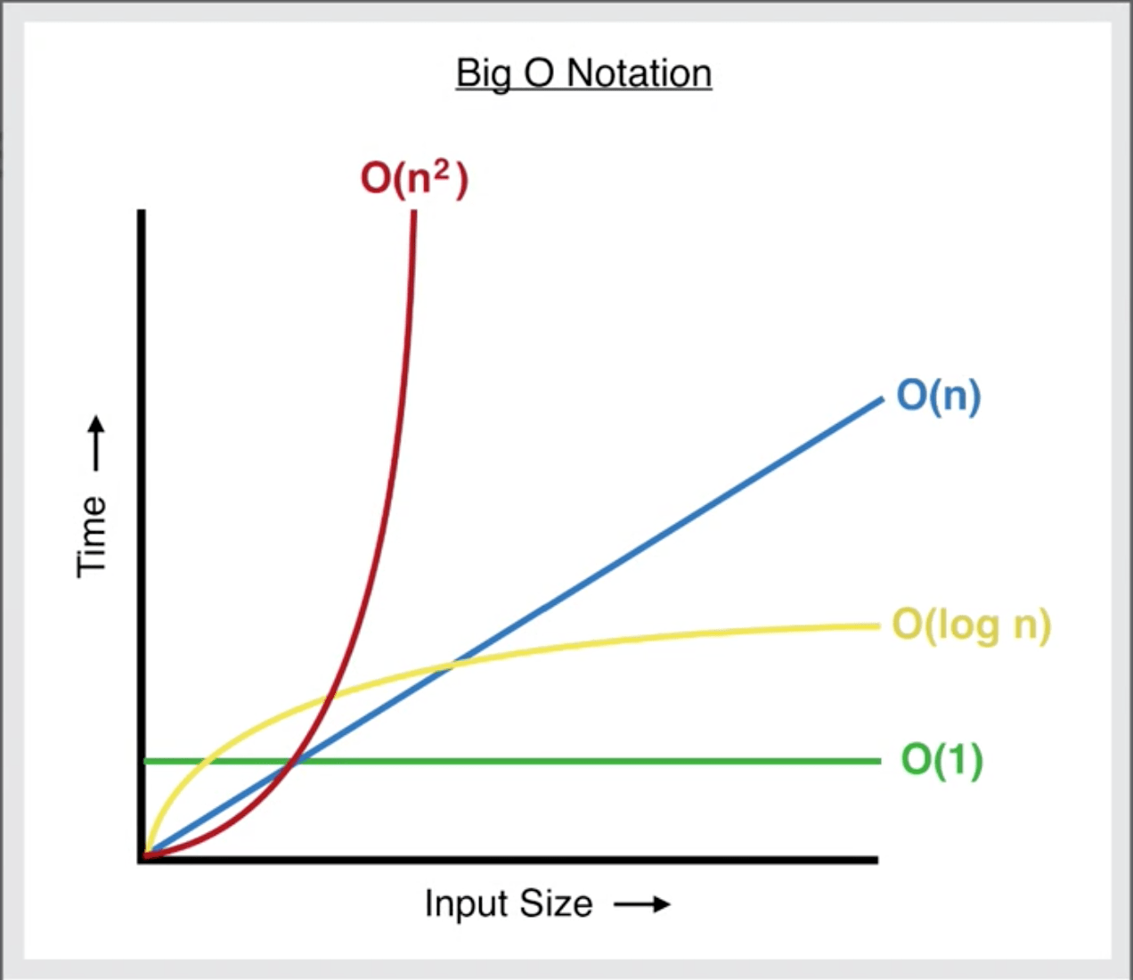
Space complexity refers to the amount of memory used by an algorithm to complete its execution, as a function of the size of the input. The space complexity of an algorithm can be affected by various factors such as the size of the input data, the data structures used in the algorithm, the number and size of temporary variables, and the recursion depth. Time complexity refers to the amount of time required by an algorithm to run as the input size grows. It is usually measured in terms of the "Big O" notation, which describes the upper bound of an algorithm's time complexity.

Why do you think a programmer should care about space and time complexity?

  • Programmers should care about space and time complexity because the amount of space and the amount of time that a program takes up depends on how efficient the program is. The less space and time the program takes up, the better the program is, but only if it completes all necessary tasks.

Take a look at our lassen volcano example from the data compression tech talk. The first code block is the original image. In the second code block, change the baseWidth to rescale the image.

from IPython.display import Image, display
from pathlib import Path 

# prepares a series of images
def image_data(path=Path("images/"), images=None):  # path of static images is defaulted
    for image in images:
        # File to open
        image['filename'] = path / image['file']  # file with path
    return images

def image_display(images):
    for image in images:  
        display(Image(filename=image['filename']))

if __name__ == "__main__":
    lassen_volcano = image_data(images=[{'source': "Peter Carolin", 'label': "Lassen Volcano", 'file': "lassen-volcano.jpg"}])
    image_display(lassen_volcano)
    
from IPython.display import HTML, display
from pathlib import Path 
from PIL import Image as pilImage 
from io import BytesIO
import base64

# prepares a series of images
def image_data(path=Path("images/"), images=None):  # path of static images is defaulted
    for image in images:
        # File to open
        image['filename'] = path / image['file']  # file with path
    return images

def scale_image(img):
    baseWidth = 625
    #baseWidth = 1250
    #baseWidth = 2500
    #baseWidth = 5000 # see the effect of doubling or halfing the baseWidth 
    #baseWidth = 10000 
    #baseWidth = 20000
    #baseWidth = 40000
    scalePercent = (baseWidth/float(img.size[0]))
    scaleHeight = int((float(img.size[1])*float(scalePercent)))
    scale = (baseWidth, scaleHeight)
    return img.resize(scale)

def image_to_base64(img, format):
    with BytesIO() as buffer:
        img.save(buffer, format)
        return base64.b64encode(buffer.getvalue()).decode()
    
def image_management(image):  # path of static images is defaulted        
    # Image open return PIL image object
    img = pilImage.open(image['filename'])
    
    # Python Image Library operations
    image['format'] = img.format
    image['mode'] = img.mode
    image['size'] = img.size
    image['width'], image['height'] = img.size
    image['pixels'] = image['width'] * image['height']
    # Scale the Image
    img = scale_image(img)
    image['pil'] = img
    image['scaled_size'] = img.size
    image['scaled_width'], image['scaled_height'] = img.size
    image['scaled_pixels'] = image['scaled_width'] * image['scaled_height']
    # Scaled HTML
    image['html'] = '<img src="data:image/png;base64,%s">' % image_to_base64(image['pil'], image['format'])


if __name__ == "__main__":
    # Use numpy to concatenate two arrays
    images = image_data(images = [{'source': "Peter Carolin", 'label': "Lassen Volcano", 'file': "lassen-volcano.jpg"}])
    
    # Display meta data, scaled view, and grey scale for each image
    for image in images:
        image_management(image)
        print("---- meta data -----")
        print(image['label'])
        print(image['source'])
        print(image['format'])
        print(image['mode'])
        print("Original size: ", image['size'], " pixels: ", f"{image['pixels']:,}")
        print("Scaled size: ", image['scaled_size'], " pixels: ", f"{image['scaled_pixels']:,}")
        
        print("-- original image --")
        display(HTML(image['html'])) 
---- meta data -----
Lassen Volcano
Peter Carolin
JPEG
RGB
Original size:  (2792, 2094)  pixels:  5,846,448
Scaled size:  (625, 468)  pixels:  292,500
-- original image --

Do you think this is a time complexity or space complexity or both problem?

  • This is both a time and space complexity problem because the larger the file, the more space it takes up and the more time it will take to load, meaning that both space and time are being put in question here.

Big O Notation

  • Constant O(1)
  • Linear O(n)
  • Quadratic O(n^2)
  • Logarithmic O(logn)
  • Exponential (O(2^n))
numbers = list(range(1000))
print(numbers)
[0, 1, 2, 3, 4, 5, 6, 7, 8, 9, 10, 11, 12, 13, 14, 15, 16, 17, 18, 19, 20, 21, 22, 23, 24, 25, 26, 27, 28, 29, 30, 31, 32, 33, 34, 35, 36, 37, 38, 39, 40, 41, 42, 43, 44, 45, 46, 47, 48, 49, 50, 51, 52, 53, 54, 55, 56, 57, 58, 59, 60, 61, 62, 63, 64, 65, 66, 67, 68, 69, 70, 71, 72, 73, 74, 75, 76, 77, 78, 79, 80, 81, 82, 83, 84, 85, 86, 87, 88, 89, 90, 91, 92, 93, 94, 95, 96, 97, 98, 99, 100, 101, 102, 103, 104, 105, 106, 107, 108, 109, 110, 111, 112, 113, 114, 115, 116, 117, 118, 119, 120, 121, 122, 123, 124, 125, 126, 127, 128, 129, 130, 131, 132, 133, 134, 135, 136, 137, 138, 139, 140, 141, 142, 143, 144, 145, 146, 147, 148, 149, 150, 151, 152, 153, 154, 155, 156, 157, 158, 159, 160, 161, 162, 163, 164, 165, 166, 167, 168, 169, 170, 171, 172, 173, 174, 175, 176, 177, 178, 179, 180, 181, 182, 183, 184, 185, 186, 187, 188, 189, 190, 191, 192, 193, 194, 195, 196, 197, 198, 199, 200, 201, 202, 203, 204, 205, 206, 207, 208, 209, 210, 211, 212, 213, 214, 215, 216, 217, 218, 219, 220, 221, 222, 223, 224, 225, 226, 227, 228, 229, 230, 231, 232, 233, 234, 235, 236, 237, 238, 239, 240, 241, 242, 243, 244, 245, 246, 247, 248, 249, 250, 251, 252, 253, 254, 255, 256, 257, 258, 259, 260, 261, 262, 263, 264, 265, 266, 267, 268, 269, 270, 271, 272, 273, 274, 275, 276, 277, 278, 279, 280, 281, 282, 283, 284, 285, 286, 287, 288, 289, 290, 291, 292, 293, 294, 295, 296, 297, 298, 299, 300, 301, 302, 303, 304, 305, 306, 307, 308, 309, 310, 311, 312, 313, 314, 315, 316, 317, 318, 319, 320, 321, 322, 323, 324, 325, 326, 327, 328, 329, 330, 331, 332, 333, 334, 335, 336, 337, 338, 339, 340, 341, 342, 343, 344, 345, 346, 347, 348, 349, 350, 351, 352, 353, 354, 355, 356, 357, 358, 359, 360, 361, 362, 363, 364, 365, 366, 367, 368, 369, 370, 371, 372, 373, 374, 375, 376, 377, 378, 379, 380, 381, 382, 383, 384, 385, 386, 387, 388, 389, 390, 391, 392, 393, 394, 395, 396, 397, 398, 399, 400, 401, 402, 403, 404, 405, 406, 407, 408, 409, 410, 411, 412, 413, 414, 415, 416, 417, 418, 419, 420, 421, 422, 423, 424, 425, 426, 427, 428, 429, 430, 431, 432, 433, 434, 435, 436, 437, 438, 439, 440, 441, 442, 443, 444, 445, 446, 447, 448, 449, 450, 451, 452, 453, 454, 455, 456, 457, 458, 459, 460, 461, 462, 463, 464, 465, 466, 467, 468, 469, 470, 471, 472, 473, 474, 475, 476, 477, 478, 479, 480, 481, 482, 483, 484, 485, 486, 487, 488, 489, 490, 491, 492, 493, 494, 495, 496, 497, 498, 499, 500, 501, 502, 503, 504, 505, 506, 507, 508, 509, 510, 511, 512, 513, 514, 515, 516, 517, 518, 519, 520, 521, 522, 523, 524, 525, 526, 527, 528, 529, 530, 531, 532, 533, 534, 535, 536, 537, 538, 539, 540, 541, 542, 543, 544, 545, 546, 547, 548, 549, 550, 551, 552, 553, 554, 555, 556, 557, 558, 559, 560, 561, 562, 563, 564, 565, 566, 567, 568, 569, 570, 571, 572, 573, 574, 575, 576, 577, 578, 579, 580, 581, 582, 583, 584, 585, 586, 587, 588, 589, 590, 591, 592, 593, 594, 595, 596, 597, 598, 599, 600, 601, 602, 603, 604, 605, 606, 607, 608, 609, 610, 611, 612, 613, 614, 615, 616, 617, 618, 619, 620, 621, 622, 623, 624, 625, 626, 627, 628, 629, 630, 631, 632, 633, 634, 635, 636, 637, 638, 639, 640, 641, 642, 643, 644, 645, 646, 647, 648, 649, 650, 651, 652, 653, 654, 655, 656, 657, 658, 659, 660, 661, 662, 663, 664, 665, 666, 667, 668, 669, 670, 671, 672, 673, 674, 675, 676, 677, 678, 679, 680, 681, 682, 683, 684, 685, 686, 687, 688, 689, 690, 691, 692, 693, 694, 695, 696, 697, 698, 699, 700, 701, 702, 703, 704, 705, 706, 707, 708, 709, 710, 711, 712, 713, 714, 715, 716, 717, 718, 719, 720, 721, 722, 723, 724, 725, 726, 727, 728, 729, 730, 731, 732, 733, 734, 735, 736, 737, 738, 739, 740, 741, 742, 743, 744, 745, 746, 747, 748, 749, 750, 751, 752, 753, 754, 755, 756, 757, 758, 759, 760, 761, 762, 763, 764, 765, 766, 767, 768, 769, 770, 771, 772, 773, 774, 775, 776, 777, 778, 779, 780, 781, 782, 783, 784, 785, 786, 787, 788, 789, 790, 791, 792, 793, 794, 795, 796, 797, 798, 799, 800, 801, 802, 803, 804, 805, 806, 807, 808, 809, 810, 811, 812, 813, 814, 815, 816, 817, 818, 819, 820, 821, 822, 823, 824, 825, 826, 827, 828, 829, 830, 831, 832, 833, 834, 835, 836, 837, 838, 839, 840, 841, 842, 843, 844, 845, 846, 847, 848, 849, 850, 851, 852, 853, 854, 855, 856, 857, 858, 859, 860, 861, 862, 863, 864, 865, 866, 867, 868, 869, 870, 871, 872, 873, 874, 875, 876, 877, 878, 879, 880, 881, 882, 883, 884, 885, 886, 887, 888, 889, 890, 891, 892, 893, 894, 895, 896, 897, 898, 899, 900, 901, 902, 903, 904, 905, 906, 907, 908, 909, 910, 911, 912, 913, 914, 915, 916, 917, 918, 919, 920, 921, 922, 923, 924, 925, 926, 927, 928, 929, 930, 931, 932, 933, 934, 935, 936, 937, 938, 939, 940, 941, 942, 943, 944, 945, 946, 947, 948, 949, 950, 951, 952, 953, 954, 955, 956, 957, 958, 959, 960, 961, 962, 963, 964, 965, 966, 967, 968, 969, 970, 971, 972, 973, 974, 975, 976, 977, 978, 979, 980, 981, 982, 983, 984, 985, 986, 987, 988, 989, 990, 991, 992, 993, 994, 995, 996, 997, 998, 999]

Constant O(1)

Time

An example of a constant time algorithm is accessing a specific element in an array. It does not matter how large the array is, accessing an element in the array takes the same amount of time. Therefore, the time complexity of this operation is constant, denoted by O(1).

print(numbers[263])

ncaa_bb_ranks = {1:"Alabama",2:"Houston", 3:"Purdue", 4:"Kansas"}
#look up a value in a dictionary given a key
print(ncaa_bb_ranks[1]) 
263
Alabama

Space

This function takes two number inputs and returns their sum. The function does not create any additional data structures or variables that are dependent on the input size, so its space complexity is constant, or O(1). Regardless of how large the input numbers are, the function will always require the same amount of memory to execute.

def sum(a, b): 
  return a + b

print(sum(90,88))
print(sum(.9,.88))
178
1.78

Linear O(n)

Time

An example of a linear time algorithm is traversing a list or an array. When the size of the list or array increases, the time taken to traverse it also increases linearly with the size. Hence, the time complexity of this operation is O(n), where n is the size of the list or array being traversed.

for i in numbers:
    print(i)

Space

This function takes a list of elements arr as input and returns a new list with the elements in reverse order. The function creates a new list reversed_arr of the same size as arr to store the reversed elements. The size of reversed_arr depends on the size of the input arr, so the space complexity of this function is O(n). As the input size increases, the amount of memory required to execute the function also increases linearly.

def reverse_list(arr):
    n = len(arr) 
    reversed_arr = [None] * n #create a list of None based on the length or arr
    for i in range(n):
        reversed_arr[n-i-1] = arr[i] #stores the value at the index of arr to the value at the index of reversed_arr starting at the beginning for arr and end for reversed_arr 
    return reversed_arr

print(numbers)
print(reverse_list(numbers))
[0, 1, 2, 3, 4, 5, 6, 7, 8, 9, 10, 11, 12, 13, 14, 15, 16, 17, 18, 19, 20, 21, 22, 23, 24, 25, 26, 27, 28, 29, 30, 31, 32, 33, 34, 35, 36, 37, 38, 39, 40, 41, 42, 43, 44, 45, 46, 47, 48, 49, 50, 51, 52, 53, 54, 55, 56, 57, 58, 59, 60, 61, 62, 63, 64, 65, 66, 67, 68, 69, 70, 71, 72, 73, 74, 75, 76, 77, 78, 79, 80, 81, 82, 83, 84, 85, 86, 87, 88, 89, 90, 91, 92, 93, 94, 95, 96, 97, 98, 99, 100, 101, 102, 103, 104, 105, 106, 107, 108, 109, 110, 111, 112, 113, 114, 115, 116, 117, 118, 119, 120, 121, 122, 123, 124, 125, 126, 127, 128, 129, 130, 131, 132, 133, 134, 135, 136, 137, 138, 139, 140, 141, 142, 143, 144, 145, 146, 147, 148, 149, 150, 151, 152, 153, 154, 155, 156, 157, 158, 159, 160, 161, 162, 163, 164, 165, 166, 167, 168, 169, 170, 171, 172, 173, 174, 175, 176, 177, 178, 179, 180, 181, 182, 183, 184, 185, 186, 187, 188, 189, 190, 191, 192, 193, 194, 195, 196, 197, 198, 199, 200, 201, 202, 203, 204, 205, 206, 207, 208, 209, 210, 211, 212, 213, 214, 215, 216, 217, 218, 219, 220, 221, 222, 223, 224, 225, 226, 227, 228, 229, 230, 231, 232, 233, 234, 235, 236, 237, 238, 239, 240, 241, 242, 243, 244, 245, 246, 247, 248, 249, 250, 251, 252, 253, 254, 255, 256, 257, 258, 259, 260, 261, 262, 263, 264, 265, 266, 267, 268, 269, 270, 271, 272, 273, 274, 275, 276, 277, 278, 279, 280, 281, 282, 283, 284, 285, 286, 287, 288, 289, 290, 291, 292, 293, 294, 295, 296, 297, 298, 299, 300, 301, 302, 303, 304, 305, 306, 307, 308, 309, 310, 311, 312, 313, 314, 315, 316, 317, 318, 319, 320, 321, 322, 323, 324, 325, 326, 327, 328, 329, 330, 331, 332, 333, 334, 335, 336, 337, 338, 339, 340, 341, 342, 343, 344, 345, 346, 347, 348, 349, 350, 351, 352, 353, 354, 355, 356, 357, 358, 359, 360, 361, 362, 363, 364, 365, 366, 367, 368, 369, 370, 371, 372, 373, 374, 375, 376, 377, 378, 379, 380, 381, 382, 383, 384, 385, 386, 387, 388, 389, 390, 391, 392, 393, 394, 395, 396, 397, 398, 399, 400, 401, 402, 403, 404, 405, 406, 407, 408, 409, 410, 411, 412, 413, 414, 415, 416, 417, 418, 419, 420, 421, 422, 423, 424, 425, 426, 427, 428, 429, 430, 431, 432, 433, 434, 435, 436, 437, 438, 439, 440, 441, 442, 443, 444, 445, 446, 447, 448, 449, 450, 451, 452, 453, 454, 455, 456, 457, 458, 459, 460, 461, 462, 463, 464, 465, 466, 467, 468, 469, 470, 471, 472, 473, 474, 475, 476, 477, 478, 479, 480, 481, 482, 483, 484, 485, 486, 487, 488, 489, 490, 491, 492, 493, 494, 495, 496, 497, 498, 499, 500, 501, 502, 503, 504, 505, 506, 507, 508, 509, 510, 511, 512, 513, 514, 515, 516, 517, 518, 519, 520, 521, 522, 523, 524, 525, 526, 527, 528, 529, 530, 531, 532, 533, 534, 535, 536, 537, 538, 539, 540, 541, 542, 543, 544, 545, 546, 547, 548, 549, 550, 551, 552, 553, 554, 555, 556, 557, 558, 559, 560, 561, 562, 563, 564, 565, 566, 567, 568, 569, 570, 571, 572, 573, 574, 575, 576, 577, 578, 579, 580, 581, 582, 583, 584, 585, 586, 587, 588, 589, 590, 591, 592, 593, 594, 595, 596, 597, 598, 599, 600, 601, 602, 603, 604, 605, 606, 607, 608, 609, 610, 611, 612, 613, 614, 615, 616, 617, 618, 619, 620, 621, 622, 623, 624, 625, 626, 627, 628, 629, 630, 631, 632, 633, 634, 635, 636, 637, 638, 639, 640, 641, 642, 643, 644, 645, 646, 647, 648, 649, 650, 651, 652, 653, 654, 655, 656, 657, 658, 659, 660, 661, 662, 663, 664, 665, 666, 667, 668, 669, 670, 671, 672, 673, 674, 675, 676, 677, 678, 679, 680, 681, 682, 683, 684, 685, 686, 687, 688, 689, 690, 691, 692, 693, 694, 695, 696, 697, 698, 699, 700, 701, 702, 703, 704, 705, 706, 707, 708, 709, 710, 711, 712, 713, 714, 715, 716, 717, 718, 719, 720, 721, 722, 723, 724, 725, 726, 727, 728, 729, 730, 731, 732, 733, 734, 735, 736, 737, 738, 739, 740, 741, 742, 743, 744, 745, 746, 747, 748, 749, 750, 751, 752, 753, 754, 755, 756, 757, 758, 759, 760, 761, 762, 763, 764, 765, 766, 767, 768, 769, 770, 771, 772, 773, 774, 775, 776, 777, 778, 779, 780, 781, 782, 783, 784, 785, 786, 787, 788, 789, 790, 791, 792, 793, 794, 795, 796, 797, 798, 799, 800, 801, 802, 803, 804, 805, 806, 807, 808, 809, 810, 811, 812, 813, 814, 815, 816, 817, 818, 819, 820, 821, 822, 823, 824, 825, 826, 827, 828, 829, 830, 831, 832, 833, 834, 835, 836, 837, 838, 839, 840, 841, 842, 843, 844, 845, 846, 847, 848, 849, 850, 851, 852, 853, 854, 855, 856, 857, 858, 859, 860, 861, 862, 863, 864, 865, 866, 867, 868, 869, 870, 871, 872, 873, 874, 875, 876, 877, 878, 879, 880, 881, 882, 883, 884, 885, 886, 887, 888, 889, 890, 891, 892, 893, 894, 895, 896, 897, 898, 899, 900, 901, 902, 903, 904, 905, 906, 907, 908, 909, 910, 911, 912, 913, 914, 915, 916, 917, 918, 919, 920, 921, 922, 923, 924, 925, 926, 927, 928, 929, 930, 931, 932, 933, 934, 935, 936, 937, 938, 939, 940, 941, 942, 943, 944, 945, 946, 947, 948, 949, 950, 951, 952, 953, 954, 955, 956, 957, 958, 959, 960, 961, 962, 963, 964, 965, 966, 967, 968, 969, 970, 971, 972, 973, 974, 975, 976, 977, 978, 979, 980, 981, 982, 983, 984, 985, 986, 987, 988, 989, 990, 991, 992, 993, 994, 995, 996, 997, 998, 999]
[999, 998, 997, 996, 995, 994, 993, 992, 991, 990, 989, 988, 987, 986, 985, 984, 983, 982, 981, 980, 979, 978, 977, 976, 975, 974, 973, 972, 971, 970, 969, 968, 967, 966, 965, 964, 963, 962, 961, 960, 959, 958, 957, 956, 955, 954, 953, 952, 951, 950, 949, 948, 947, 946, 945, 944, 943, 942, 941, 940, 939, 938, 937, 936, 935, 934, 933, 932, 931, 930, 929, 928, 927, 926, 925, 924, 923, 922, 921, 920, 919, 918, 917, 916, 915, 914, 913, 912, 911, 910, 909, 908, 907, 906, 905, 904, 903, 902, 901, 900, 899, 898, 897, 896, 895, 894, 893, 892, 891, 890, 889, 888, 887, 886, 885, 884, 883, 882, 881, 880, 879, 878, 877, 876, 875, 874, 873, 872, 871, 870, 869, 868, 867, 866, 865, 864, 863, 862, 861, 860, 859, 858, 857, 856, 855, 854, 853, 852, 851, 850, 849, 848, 847, 846, 845, 844, 843, 842, 841, 840, 839, 838, 837, 836, 835, 834, 833, 832, 831, 830, 829, 828, 827, 826, 825, 824, 823, 822, 821, 820, 819, 818, 817, 816, 815, 814, 813, 812, 811, 810, 809, 808, 807, 806, 805, 804, 803, 802, 801, 800, 799, 798, 797, 796, 795, 794, 793, 792, 791, 790, 789, 788, 787, 786, 785, 784, 783, 782, 781, 780, 779, 778, 777, 776, 775, 774, 773, 772, 771, 770, 769, 768, 767, 766, 765, 764, 763, 762, 761, 760, 759, 758, 757, 756, 755, 754, 753, 752, 751, 750, 749, 748, 747, 746, 745, 744, 743, 742, 741, 740, 739, 738, 737, 736, 735, 734, 733, 732, 731, 730, 729, 728, 727, 726, 725, 724, 723, 722, 721, 720, 719, 718, 717, 716, 715, 714, 713, 712, 711, 710, 709, 708, 707, 706, 705, 704, 703, 702, 701, 700, 699, 698, 697, 696, 695, 694, 693, 692, 691, 690, 689, 688, 687, 686, 685, 684, 683, 682, 681, 680, 679, 678, 677, 676, 675, 674, 673, 672, 671, 670, 669, 668, 667, 666, 665, 664, 663, 662, 661, 660, 659, 658, 657, 656, 655, 654, 653, 652, 651, 650, 649, 648, 647, 646, 645, 644, 643, 642, 641, 640, 639, 638, 637, 636, 635, 634, 633, 632, 631, 630, 629, 628, 627, 626, 625, 624, 623, 622, 621, 620, 619, 618, 617, 616, 615, 614, 613, 612, 611, 610, 609, 608, 607, 606, 605, 604, 603, 602, 601, 600, 599, 598, 597, 596, 595, 594, 593, 592, 591, 590, 589, 588, 587, 586, 585, 584, 583, 582, 581, 580, 579, 578, 577, 576, 575, 574, 573, 572, 571, 570, 569, 568, 567, 566, 565, 564, 563, 562, 561, 560, 559, 558, 557, 556, 555, 554, 553, 552, 551, 550, 549, 548, 547, 546, 545, 544, 543, 542, 541, 540, 539, 538, 537, 536, 535, 534, 533, 532, 531, 530, 529, 528, 527, 526, 525, 524, 523, 522, 521, 520, 519, 518, 517, 516, 515, 514, 513, 512, 511, 510, 509, 508, 507, 506, 505, 504, 503, 502, 501, 500, 499, 498, 497, 496, 495, 494, 493, 492, 491, 490, 489, 488, 487, 486, 485, 484, 483, 482, 481, 480, 479, 478, 477, 476, 475, 474, 473, 472, 471, 470, 469, 468, 467, 466, 465, 464, 463, 462, 461, 460, 459, 458, 457, 456, 455, 454, 453, 452, 451, 450, 449, 448, 447, 446, 445, 444, 443, 442, 441, 440, 439, 438, 437, 436, 435, 434, 433, 432, 431, 430, 429, 428, 427, 426, 425, 424, 423, 422, 421, 420, 419, 418, 417, 416, 415, 414, 413, 412, 411, 410, 409, 408, 407, 406, 405, 404, 403, 402, 401, 400, 399, 398, 397, 396, 395, 394, 393, 392, 391, 390, 389, 388, 387, 386, 385, 384, 383, 382, 381, 380, 379, 378, 377, 376, 375, 374, 373, 372, 371, 370, 369, 368, 367, 366, 365, 364, 363, 362, 361, 360, 359, 358, 357, 356, 355, 354, 353, 352, 351, 350, 349, 348, 347, 346, 345, 344, 343, 342, 341, 340, 339, 338, 337, 336, 335, 334, 333, 332, 331, 330, 329, 328, 327, 326, 325, 324, 323, 322, 321, 320, 319, 318, 317, 316, 315, 314, 313, 312, 311, 310, 309, 308, 307, 306, 305, 304, 303, 302, 301, 300, 299, 298, 297, 296, 295, 294, 293, 292, 291, 290, 289, 288, 287, 286, 285, 284, 283, 282, 281, 280, 279, 278, 277, 276, 275, 274, 273, 272, 271, 270, 269, 268, 267, 266, 265, 264, 263, 262, 261, 260, 259, 258, 257, 256, 255, 254, 253, 252, 251, 250, 249, 248, 247, 246, 245, 244, 243, 242, 241, 240, 239, 238, 237, 236, 235, 234, 233, 232, 231, 230, 229, 228, 227, 226, 225, 224, 223, 222, 221, 220, 219, 218, 217, 216, 215, 214, 213, 212, 211, 210, 209, 208, 207, 206, 205, 204, 203, 202, 201, 200, 199, 198, 197, 196, 195, 194, 193, 192, 191, 190, 189, 188, 187, 186, 185, 184, 183, 182, 181, 180, 179, 178, 177, 176, 175, 174, 173, 172, 171, 170, 169, 168, 167, 166, 165, 164, 163, 162, 161, 160, 159, 158, 157, 156, 155, 154, 153, 152, 151, 150, 149, 148, 147, 146, 145, 144, 143, 142, 141, 140, 139, 138, 137, 136, 135, 134, 133, 132, 131, 130, 129, 128, 127, 126, 125, 124, 123, 122, 121, 120, 119, 118, 117, 116, 115, 114, 113, 112, 111, 110, 109, 108, 107, 106, 105, 104, 103, 102, 101, 100, 99, 98, 97, 96, 95, 94, 93, 92, 91, 90, 89, 88, 87, 86, 85, 84, 83, 82, 81, 80, 79, 78, 77, 76, 75, 74, 73, 72, 71, 70, 69, 68, 67, 66, 65, 64, 63, 62, 61, 60, 59, 58, 57, 56, 55, 54, 53, 52, 51, 50, 49, 48, 47, 46, 45, 44, 43, 42, 41, 40, 39, 38, 37, 36, 35, 34, 33, 32, 31, 30, 29, 28, 27, 26, 25, 24, 23, 22, 21, 20, 19, 18, 17, 16, 15, 14, 13, 12, 11, 10, 9, 8, 7, 6, 5, 4, 3, 2, 1, 0]

Quadratic O(n^2)

Time

An example of a quadratic time algorithm is nested loops. When there are two nested loops that both iterate over the same collection, the time taken to complete the algorithm grows quadratically with the size of the collection. Hence, the time complexity of this operation is O(n^2), where n is the size of the collection being iterated over.

for i in numbers:
    for j in numbers:
        print(i,j)

Space

This function takes two matrices matrix1 and matrix2 as input and returns their product as a new matrix. The function creates a new matrix result with dimensions m by n to store the product of the input matrices. The size of result depends on the size of the input matrices, so the space complexity of this function is O(n^2). As the size of the input matrices increases, the amount of memory required to execute the function also increases quadratically.

Example of Matrix Multiplication

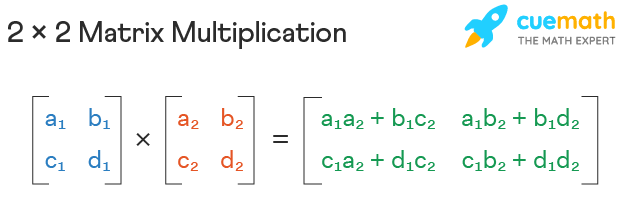
  • Main take away is that a new matrix is created.
def multiply_matrices(matrix1, matrix2):
    m = len(matrix1) 
    n = len(matrix2[0])
    result = [[0] * n] * m #this creates the new matrix based on the size of matrix 1 and 2
    for i in range(m):
        for j in range(n):
            for k in range(len(matrix2)):
                result[i][j] += matrix1[i][k] * matrix2[k][j]
    return result

print(multiply_matrices([[1,2],[3,4]], [[3,4],[1,2]]))
[[18, 28], [18, 28]]

Logarithmic O(logn)

Time

An example of a log time algorithm is binary search. Binary search is an algorithm that searches for a specific element in a sorted list by repeatedly dividing the search interval in half. As a result, the time taken to complete the search grows logarithmically with the size of the list. Hence, the time complexity of this operation is O(log n), where n is the size of the list being searched.

def binary_search(arr, low, high, target):
    while low <= high:
        mid = (low + high) // 2 #integer division
        if arr[mid] == target:
            return mid
        elif arr[mid] < target:
            low = mid + 1
        else:
            high = mid - 1

target = 263
result = binary_search(numbers, 0, len(numbers) - 1, target)

print(result)
263

Space

The same algorithm above has a O(logn) space complexity. The function takes an array arr, its lower and upper bounds low and high, and a target value target. The function searches for target within the bounds of arr by recursively dividing the search space in half until the target is found or the search space is empty. The function does not create any new data structures that depend on the size of arr. Instead, the function uses the call stack to keep track of the recursive calls. Since the maximum depth of the recursive calls is O(logn), where n is the size of arr, the space complexity of this function is O(logn). As the size of arr increases, the amount of memory required to execute the function grows logarithmically.

Exponential O(2^n)

Time

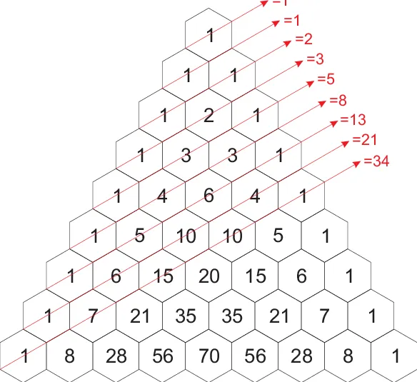
An example of an O(2^n) algorithm is the recursive implementation of the Fibonacci sequence. The Fibonacci sequence is a series of numbers where each number is the sum of the two preceding ones, starting from 0 and 1. The recursive implementation of the Fibonacci sequence calculates each number by recursively calling itself with the two preceding numbers until it reaches the base case (i.e., the first or second number in the sequence). The algorithm takes O(2^n) time in the worst case because it has to calculate each number in the sequence by making two recursive calls.

A visualization of calculating the fibonacci sequence

def fibonacci(n):
    if n <= 1:
        return n
    else:
        return fibonacci(n-1) + fibonacci(n-2)

#print(fibonacci(5))
#print(fibonacci(10))
#print(fibonacci(20))
#print(fibonacci(30))
print(fibonacci(40))
102334155

Space

This function takes a set s as input and generates all possible subsets of s. The function does this by recursively generating the subsets of the set without the first element, and then adding the first element to each of those subsets to generate the subsets that include the first element. The function creates a new list for each recursive call that stores the subsets, and each element in the list is a new list that represents a subset. The number of subsets that can be generated from a set of size n is 2^n, so the space complexity of this function is O(2^n). As the size of the input set increases, the amount of memory required to execute the function grows exponentially.

def generate_subsets(s):
    if not s:
        return [[]]
    subsets = generate_subsets(s[1:])
    return [[s[0]] + subset for subset in subsets] + subsets

print(generate_subsets([1,2,3]))
#print(generate_subsets(numbers))
[[1, 2, 3], [1, 2], [1, 3], [1], [2, 3], [2], [3], []]

Using the time library, we are able to see the difference in time it takes to calculate the fibonacci function above.

  • Based on what is known about the other time complexities, hypothesize the resulting elapsed time if the function is replaced.
    • The first section of code will probably take a shorter amount of time than the second section of code, however the difference shouldn't be very large. If the function were to be replaced, the time should shorten or lengthen based on the size of the fibonacci sequence.
import time

start_time = time.time()
print(fibonacci(34))
end_time = time.time()

total_time = end_time - start_time
print("Time taken:", total_time, "seconds")

start_time = time.time()
print(fibonacci(35))
end_time = time.time()

total_time = end_time - start_time
print("Time taken:", total_time, "seconds")
5702887
Time taken: 2.025815963745117 seconds
9227465
Time taken: 3.5262391567230225 seconds

Hacks

  • Record your findings when testing the time elapsed of the different algorithms.
    • O(1) is usually the algorithm that takes the least amount of time and stays the most consistent with size.
    • O(n^2) is good for small sizes in terms of time but gets bad when the input size becomes large.
    • O(n) is the second best when it comes to small sizes but it stays constant and is also the second worse when the size increases. Time is proportional to the size.
    • O(log n) is the worst for small sizes but is the best for large sizes in terms of time.
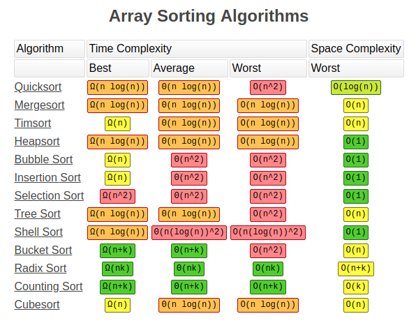
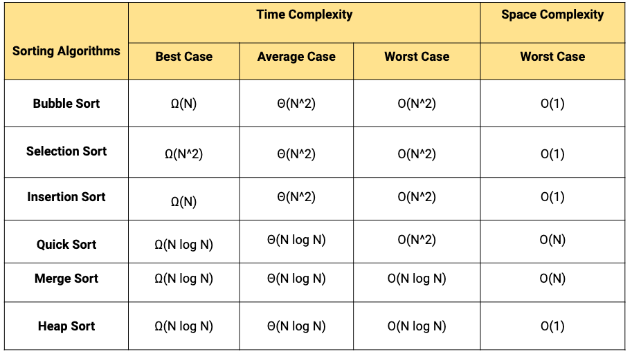
  • Although we will go more in depth later, time complexity is a key concept that relates to the different sorting algorithms. Do some basic research on the different types of sorting algorithms and their time complexity.
    • onotation
    • This image shows the size versus time each type of sorting algorithm takes up. This is useful when programming and determining which algorithm will be the more efficient to use in certain situations.
    • ntiatoin
    • notaitno
  • Why is time and space complexity important when choosing an algorithm?
    • Time and space is important when choosing an algorithm because you want to have an algorithm that is appropriate for the size that you are dealing with in order to get the best time results.
  • Should you always use a constant time algorithm / Should you never use an exponential time algorithm? Explain?
    • Constant time algorithms are good for any application but exponential ones are only good for specific applications. For small sizes, exponential are better but for larger ones the program becomes very slow and causes problems. With constant time algorithms, although they are bad for small file sizes, the are good for large ones.
  • What are some general patterns that you noticed to determine each algorithm's time and space complexity?
    • Exponential algorithms usually handle large sizes poorly and slow down as a result, causing there to be a loss in efficiency. The was that algorithms are notated is that as time goes on, the size of the program causes there to be less or more time needed for a program to run.

Complete the Time and Space Complexity analysis questions linked below. Practice